
Region Manifold Extraction#
Introduction#

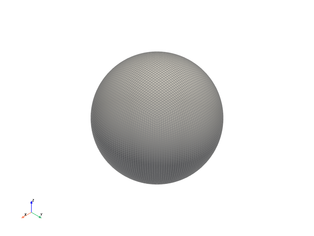
Fig. 4: Cubed-Sphere#
In this tutorial we use unstructured cubed-sphere sample data from the pantry to explore mesh regional extraction using a geodesic manifold.
Let’s Go!#
The Met Office is migrating to a unstructured cubed-sphere quadrilateral-cell mesh, which is a gridded cube projected onto a sphere i.e., there are 6 panels on the sphere, see Fig. 4:.
Each cubed-sphere is defined by the number of cells squared within each panel. In this tutorial we’ll use a C48 cubed-sphere, so there are 48 * 48 cells per panel, and 6 * 48 * 48 cells in a mesh overall.
First, let’s import geovista and generate some LFRic Model LFRic Model - For further information refer to LFRic - a modelling system fit for future computers. cubed-sphere sample data using the lfric() and lfric_sst() convenience functions:
1import geovista as gv
2from geovista.pantry.meshes import lfric, lfric_sst
As the lfric() and lfric_sst() functions both return a pyvista.PolyData we can simply use the pyvista.DataSet.plot method to render them:
1c48 = lfric(resolution="c48")
2c48.plot(show_edges=True)
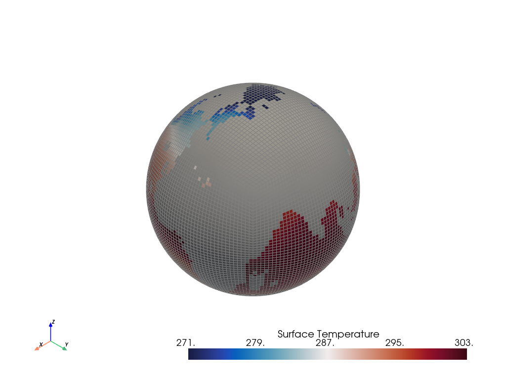
Now create the same C48 cubed-sphere resolution mesh, but this time with cells populated with Sea Surface Temperature (SST) data. Note that the land masses are masked, as this is an oceanographic dataset. Masked cells within the mesh will have nan values:
1c48_sst = lfric_sst()
2c48_sst.plot(show_edges=True)
Attention
Our goal is to extract all cubed-sphere cells within the panel covering the Americas.
We can achieve this using the geovista.geodesic.panel() function.
The panel() function is a convenience which allows you to extract cells from a mesh within 1 of the 6 named cubed-sphere panels i.e., africa, americas, antarctic, arctic, asia, and pacific.
It returns a geovista.geodesic.BBox instance, which defines a geodesic bounding-box manifold for the requested spatial region.
Hint
You can use BBox directly to create generic geodesic bounding-box manifolds.
So let’s go ahead and create the BBox for the americas cubed-sphere panel and use its mesh() method to visualise the manifold:
1from geovista.geodesic import panel
2
3americas_bbox = panel("americas")
4americas_bbox.mesh.plot(color="orange")
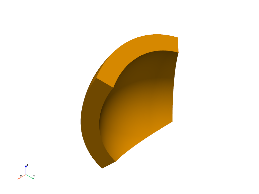
Note that the americas_bbox is constructed from geodesic lines i.e., great circles, and is a 3D manifold i.e., a water-tight geometric structure. As such, we can then use it to extract points/cells from any underlying mesh.
Before doing that, first let’s render the americas_bbox and the c48_sst mesh together so that we can see their relationship to one another and convince ourselves that the americas_bbox instance is indeed covering the correct panel of the cubed-sphere:
1p = gv.GeoPlotter()
2
3p.add_mesh(c48_sst, show_edges=True)
4p.add_mesh(americas_bbox.mesh, color="orange")
5
6p.view_yz()
7p.camera.zoom(1.2)
8p.add_axes()
9p.show()
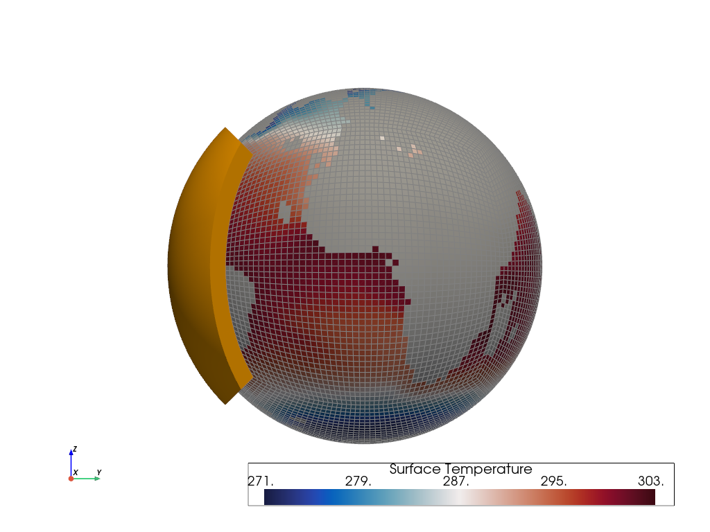
Seems to be right on the money! 👍
Note
p is a GeoPlotter instance. It inherits all the behaviour of a pyvista.Plotter, but also additional cartographic conveniences from our GeoPlotterBase.
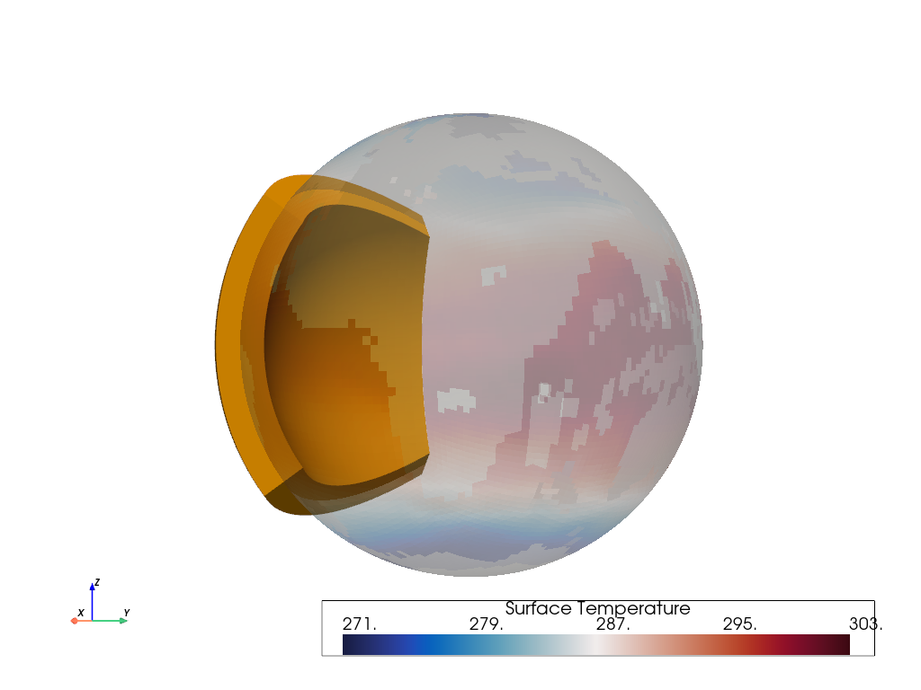
However, let’s apply some opacity to the c48_sst mesh so that we can see through the surface and view the americas_bbox from a different angle.
We’ll also use the view_poi() method to perform some cartographic camera controls on the rendered scene. Namey, move the camera to 30°E longitude.
1p = gv.GeoPlotter()
2p.add_mesh(c48_sst, opacity=0.3)
3p.add_mesh(americas_bbox.mesh, color="orange")
4
5p.view_poi(x=30)
6
7p.camera.zoom(1.2)
8p.add_axes()
9p.show()
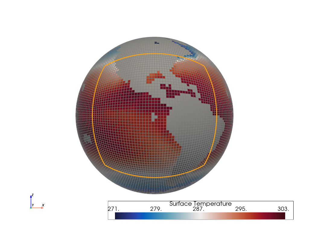
Rather than viewing the entire bounding-box, sometimes it’s more helpful to see only the boundary where the manifold intersects the surface of the mesh that it’s enclosing.
We can achieve this by using the geovista.geodesic.BBox.boundary() method:
1p = gv.GeoPlotter()
2p.add_mesh(c48_sst, show_edges=True)
3
4p.add_mesh(americas_bbox.boundary(), color="orange", line_width=5)
5
6p.view_xz()
7p.camera.zoom(1.2)
8p.add_axes()
9p.show()
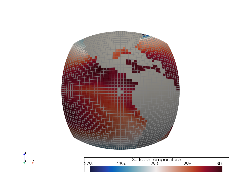
Okay, so let’s finally use the americas_bbox to extract cells from the c48_sst mesh by using the geovista.geodesic.BBox.enclosed() method:
1region = americas_bbox.enclosed(c48_sst)
The extracted region returned by enclosed() You may want to experiment with the preference kwarg of the enclosed() method to see the impact on the end result. is a pyvista.PolyData. Under the hood enclosed() uses the pyvista.DataSetFilters.select_enclosed_points() method to achieve this.
Anyways, let’s go ahead and see the extracted region, which should represent all the cells from the c48_sst mesh within the americas bounding-box:
1p = gv.GeoPlotter()
2
3p.add_mesh(region, show_edges=True)
4
5p.view_xz()
6p.add_axes()
7p.show()
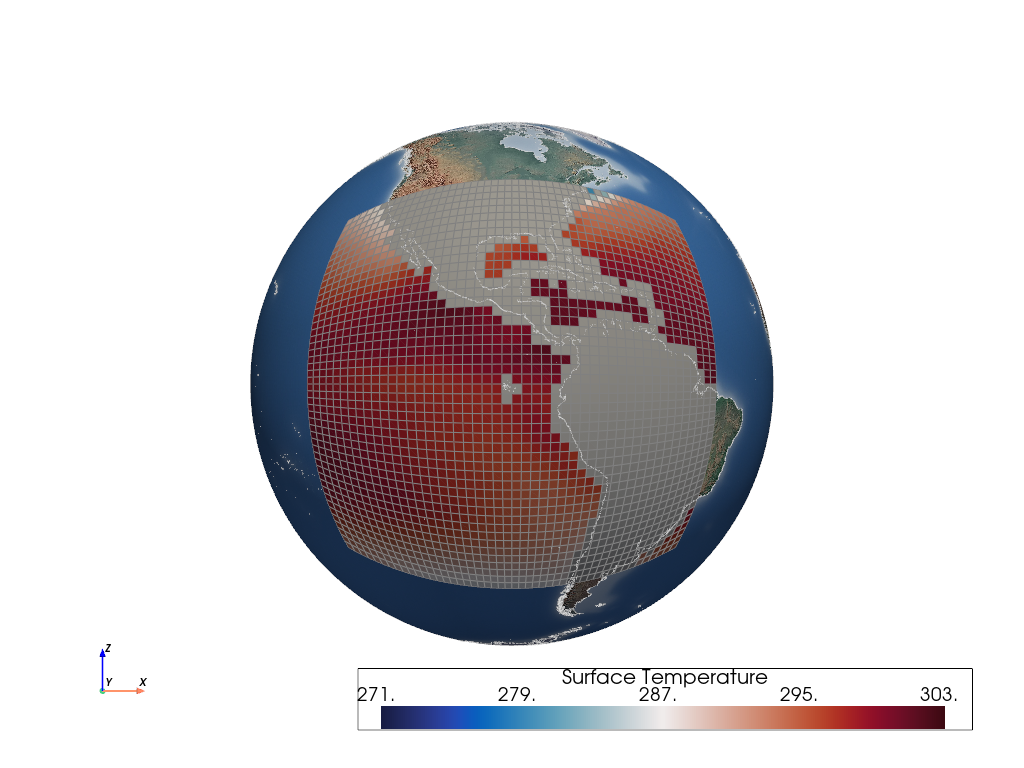
Now bring this all together by rendering the extracted region When you extract data from a mesh use the add_mesh() clim kwarg to ensure the same colorbar range. Compare this render of the region mesh with the previous render without clim. Notice the difference? along with a Natural Earth texture mapped base layer and coastlines:
 1clim = (271, 303)
 2
 3p = gv.GeoPlotter()
 4p.add_mesh(region, show_edges=True, clim=clim)
 5
 6p.add_base_layer(texture=gv.natural_earth_hypsometric())
 7p.add_coastlines(resolution="10m")
 8
 9p.view_xz()
10p.camera.zoom(1.2)
11p.show_axes()
12p.show()
As we’re not particularly interested in the masked land masses, we can easily remove them using the pyvista.DataSetFilters.threshold() method available on the region PolyData instance.
By default, the threshold() method will remove cells with nan values from the active scalars array Discover the data arrays available on a mesh with array_names, and the active scalars with active_scalars_name. on the mesh, which is just what we need:
1sea_region = region.threshold()
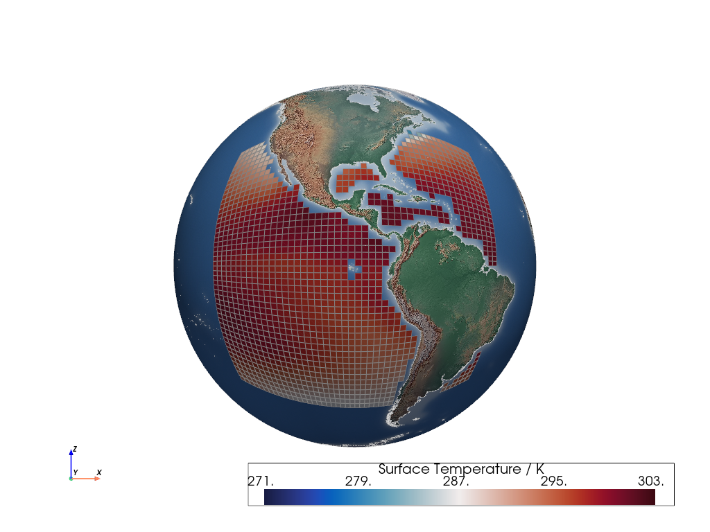
Now let’s respin the render, but with the sea_region mesh and add some S.I. units to the scalar bar:
 1p = gv.GeoPlotter()
 2
 3sargs = {"title": f"{sea_region.active_scalars_name} / K"}
 4p.add_mesh(sea_region, show_edges=True, clim=clim, scalar_bar_args=sargs)
 5
 6p.add_base_layer(texture=gv.natural_earth_hypsometric())
 7p.add_coastlines(resolution="10m")
 8p.view_xz()
 9p.camera.zoom(1.2)
10p.show_axes()
11p.show()
Extension#
geovista offers basic support for Cylindrical and Pseudo-Cylindrical cartographic projections. We’re working on maturing this capability, and later extending to other classes of projections, such as Azimuthal and Conic.
To exercise this, let’s transform our sea_region mesh to a Robinson projection using a PROJ string to define the Coordinate Reference System (CRS):
1crs = "+proj=robin lon_0=-90"
We pass the crs as a kwarg to the GeoPlotter If no crs is provided to GeoPlotter, it will assume geographic longitude and latitudes (WGS84), and render the mesh on a sphere. and render the projected scene:
1p = gv.GeoPlotter(crs=crs)
2p.add_mesh(sea_region, show_edges=True, clim=clim)
3p.add_base_layer(texture=gv.natural_earth_hypsometric())
4p.add_coastlines(resolution="10m")
5p.view_xy()
6p.camera.zoom(1.5)
7p.show_axes()
8p.show()
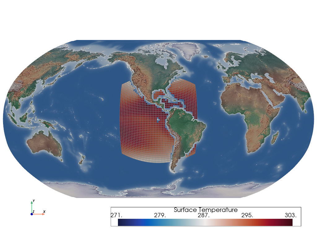
Note that the base layer and coastlines are also automatically transformed to the target projection.
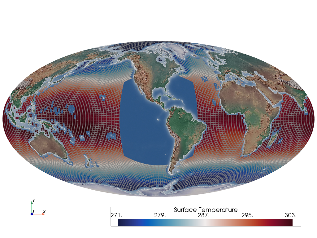
geovista also has an understanding of cartopy CRS’s. So let’s use cartopy to create a Mollweide CRS:
1import cartopy.crs as ccrs
2
3crs = ccrs.Mollweide(central_longitude=-90)
Before we use this CRS, let’s invert the sea_region i.e., find all cells not enclosed by the americas_bbox manifold. We can easily do this using the outside kwarg of enclosed():
1outside = americas_bbox.enclosed(c48_sst, outside=True)
2sea_outside = outside.threshold()
Now let’s see the final projected result:
1p = gv.GeoPlotter(crs=crs)
2p.add_mesh(sea_outside, show_edges=True, clim=clim)
3p.add_base_layer(texture=gv.natural_earth_hypsometric())
4p.add_coastlines(resolution="10m")
5p.view_xy()
6p.camera.zoom(1.5)
7p.show_axes()
8p.show()
Summary#
Key learning points of this tutorial:
using the
geovista.pantryto generate meshescreating a geodesic bounding-box manifold with
panel()introduction to the
BBoxclass and using itsboundary(),enclosed(), andmesh()methodscartographic positioning of the camera with
view_poi()performing a cell
threshold()of a mesh