クイックスタート

Estimated reading time: 14 minutes

Now that you've installed geovista, let's take a quick tour to see some of the features and capabilities on offer.

Resources

便利なように、 geovista には、ラスター、 VTK メッシュ、 Natural Earth Features 、様々な地球科学のサンプルデータなど、ビジュアライゼーションの旅を始めるのに役立つ あらかじめ用意されたリソース が付属しています。

geovistaは **バージョン管理された リソースを必要な時に自動的にダウンロードします。 しかし、すべての geovista リソースをダウンロードしてキャッシュし、オフラインで利用できるようにしたい場合は、コマンドラインで以下のように実行するだけです:

$ geovista download --all

To view the manifest of registered resources:

$ geovista download --list

注釈

もっと知りたい？

$ geovista download --help

例

注釈

Interactive Scene vtk.js は、テキストやポイントを球体としてレンダリングすることをサポートして いません 。

Let's explore some atmospheric and oceanographic model data using geovista, which makes it easy to visualize rectilinear, curvilinear, and unstructured meshes.

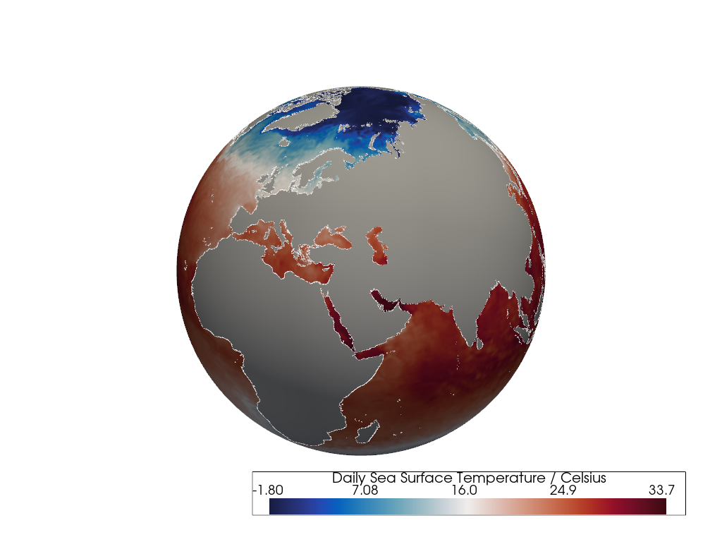
OISST AVHRR

This example renders a 2D data array with 1D X and Y rectilinear coordinates as a mesh of quadrilateral cells in 3D with coastlines.

The data source is a NOAA/NCEI Optimum Interpolation SST (OISST) Advanced Very High Resolution Radiometer (AVHRR) rectilinear grid containing 1,036,800 quadrilateral cells and 1,038,961 points.

The mesh is created from the bounds of 1D geographic longitude and latitude coordinates using the from_1d() method. Each X and Y coordinate has 2 coordinate bounds describing a quadrilateral cell.

A 2D array of Sea Surface Temperature data located on the mesh cells are rendered using the perceptually uniform cmocean balance diverging colormap, along with 10m Natural Earth coastlines. Note that the land cells are masked.

import geovista as gv
from geovista.pantry.data import oisst_avhrr_sst

# Load sample data.
sample = oisst_avhrr_sst()

# Create the mesh from the sample data.
mesh = gv.Transform.from_1d(
    sample.lons,
    sample.lats,
    data=sample.data
)

# Plot the mesh with coastlines.
p = gv.GeoPlotter()
sargs = {"title": f"{sample.name} / {sample.units}"}
p.add_mesh(
    mesh,
    cmap="balance",
    scalar_bar_args=sargs
)
p.add_coastlines(color="white")
p.camera.zoom(1.2)
p.show()

Static Scene

Interactive Scene

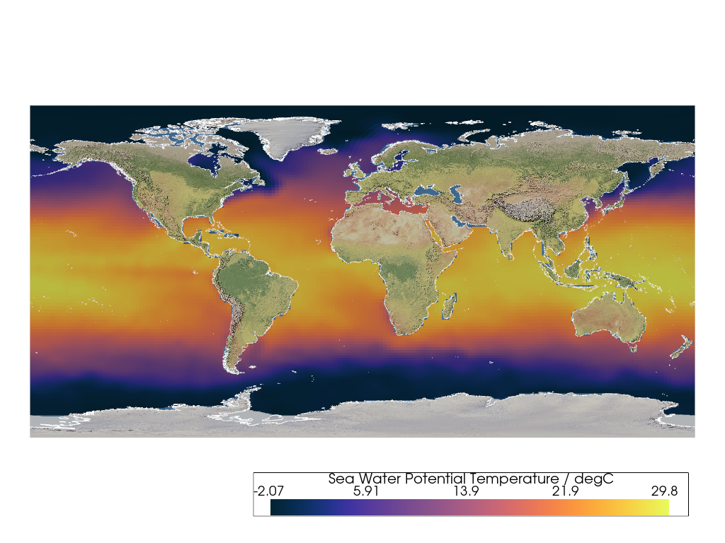
NEMO ORCA2

This example renders a 2D data array with 2D X and Y curvilinear coordinates as a mesh of quadilateral cells in 3D. A threshold is applied to remove cells with masked data. Coastlines and a base layer are also added before the results are transformed to a flat 2D surface with a Plate Carrée projection.

The data source is a Nucleus for European Modelling of the Ocean (NEMO) ORCA2 global ocean tripolar curvilinear grid containing 26,640 quadrilateral cells and 106,560 points.

As the grid is curvilinear, it is created from the bounds of 2D geographic longitude and latitude coordinates using the from_2d() method. Each X and Y coordinate has 4 coordinate bounds describing a quadrilateral cell.

As ORCA2 is an ocean model, we use a threshold to remove 10,209 nan land mask cells , and texture map a base layer underneath with a 1:50m Natural Earth I raster.

A perceptually uniform cmocean thermal colormap is used to render the Sea Water Potential Temperature data located on the grid cells, which is then complemented with 10m Natural Earth coastlines.

Finally, a cartopy CRS is used to transform the actors in the scene to the Equidistant Cylindrical (Plate Carrée) conformal cylindrical projection.

注釈

Basic projection support is available within geovista for Cylindrical and Pseudo-Cylindrical projections. As geovista matures, we'll aim to enrich that capability and complement it with other classes of projections, such as Azimuthal and Conic.

import cartopy.crs as ccrs

import geovista as gv
from geovista.pantry.data import nemo_orca2

# Load sample data.
sample = nemo_orca2()

# Create the mesh from the sample data.
mesh = gv.Transform.from_2d(
    sample.lons,
    sample.lats,
    data=sample.data
)

# Remove cells from the mesh with NaN values.
mesh = mesh.threshold()

# Plot the mesh on a Plate Carrée projection using a cartopy CRS.
p = gv.GeoPlotter(crs=ccrs.PlateCarree())
sargs = {"title": f"{sample.name} / {sample.units}"}
p.add_mesh(
    mesh,
    cmap="thermal",
    scalar_bar_args=sargs
)
p.add_base_layer(texture=gv.natural_earth_1())
p.add_coastlines(color="white")
p.view_xy()
p.camera.zoom(1.4)
p.show()

Static Scene

Interactive Scene

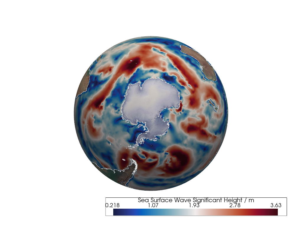
WAVEWATCH III

geovista provides rich support for easily constructing a mesh surface from various unstructured Earth Science model data.

To demonstrate this we create a WAVEWATCH III (WW3) unstructured triangular mesh from 1D X and Y unstructured coordinates and 2D connectivity using the from_unstructured() method.

The sample.connectivity, with shape (30559, 3), is used to index into the 16,160 1D geographical longitude and latitude points to create a mesh containing 30,559 triangular cells.

A 1D array of Sea Surface Wave Significant Height data is located on the mesh nodes, which is then interpolated across the mesh cells and rendered with the perceptually uniform cmocean balance divergent colormap.

As the WAVEWATCH III contains no land based cells, the 1:50m Natural Earth Cross-Blended Hypsometric Tints texture mapped base layer is visible underneath without the need to threshold the mesh.

Finally, the render is decorated with 10m Natural Earth coastlines.

import geovista as gv
from geovista.pantry.data import ww3_global_tri

# Load the sample data.
sample = ww3_global_tri()

# Create the mesh from the sample data.
mesh = gv.Transform.from_unstructured(
    sample.lons,
    sample.lats,
    connectivity=sample.connectivity,
    data=sample.data,
)

# Plot the mesh.
p = gv.GeoPlotter()
sargs = {"title": f"{sample.name} / {sample.units}"}
p.add_mesh(
    mesh,
    cmap="balance",
    scalar_bar_args=sargs
)
p.add_coastlines(color="white")
p.add_base_layer(texture=gv.natural_earth_hypsometric())
p.view_xy(negative=True)
p.camera.zoom(1.2)
p.show()

Static Scene

Interactive Scene

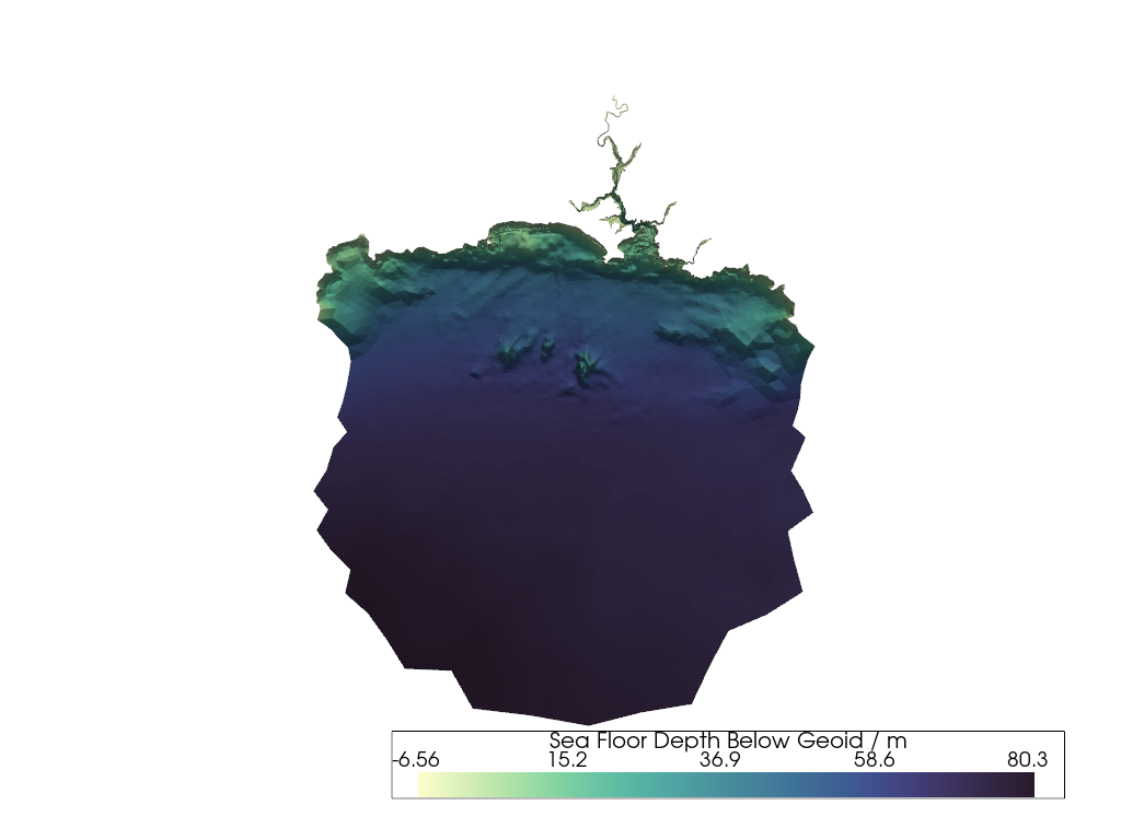
Finite Volume Community Ocean Model

This final example showcases how PyVista can take visualization of Earth Science data to the next dimension, quite literally.

We use Finite Volume Community Ocean Model (FVCOM) data to create an extruded mesh of the Plymouth Sound and Tamar River bathymetry in Cornwall, England.

First the from_unstructured() method is used to create a triangular mesh from 1D X and Y unstructured coordinates and 2D connectivity.

A 1D array of Sea Floor Depth Below Geoid data is added to the mesh cells, but also the mesh points, which are then used to displace the mesh points by a proportionally scaled amount in the direction of the mesh surface normals.

This displacement or warping of the mesh reveals the relief of the river and sea floor bathymetry, which we are then free to explore interactively.

import geovista as gv
from geovista.pantry.data import fvcom_tamar

# Load the sample data.
sample = fvcom_tamar()

# Create the mesh from the sample data.
mesh = gv.Transform.from_unstructured(
    sample.lons,
    sample.lats,
    connectivity=sample.connectivity,
    data=sample.face,
    name="face",
)

# Warp the mesh nodes by the bathymetry.
mesh.point_data["node"] = sample.node
mesh.compute_normals(cell_normals=False, point_normals=True, inplace=True)
mesh.warp_by_scalar(scalars="node", inplace=True, factor=2e-5)

# Plot the mesh.
p = gv.GeoPlotter()
sargs = {"title": f"{sample.name} / {sample.units}"}
p.add_mesh(
    mesh,
    cmap="deep",
    scalar_bar_args=sargs
)
p.view_poi()
p.show()

Static Scene

Interactive Scene

And Finally ...

この geovista 旋風ツアーが、あなたの食欲を刺激してくれることを願っています!

If so, then let's explore the next steps on your geovista journey.